Regressions and variational calculus
I found this cool post and I thought it could be fun to implement the solution as well as go over my own understanding of the derived equations.
In machine learning models we typically minimize the following loss function:
\[\text{arg min}_{f} \sum_{i = 1}^{n} \{ f(x_i) - y_i \}^2\]where the function $f$ is an estimator of $y$ . Different machine learning models propose different strategies to minimize the above loss function. However, I always wondered how to convert this optimization problem into a calculus of variation problem. It turns out that you can use the Dirac delta function.
Let $\delta_{\sigma}(x_i - \mu)$ be a function such that:
\[\delta_{\sigma}(x_i - \mu) \approx \begin{cases} 1, & \text{if $x_i = \mu$ }.\\ 0, & \text{otherwise}. \end{cases}\]The way this function works is by having a distribution around $x_i$ when $x_i$ approaches $\mu$ . This peak can be depicted by a Gaussian distribution. That is,
\[\delta_{\sigma}(x_i - \mu) = \frac{1}{\sqrt{2\pi \sigma^2 }} \exp\{ -\frac{1}{2\sigma^2} (x_i - \mu)^2 \} \text{ .}\]Then, the key insight is to make the loss function stop depending on $x_i$ and make it depend on $\mu$ instead, such that we define the following functional:
\[\begin{align} J[f] & = \sum_{i = 1}^{n} \{ f(x_i) - y_i \}^2 \\ & \approx \int_{\mathbb{R}} \sum_{i = 1}^{n} \left\{ f(\mu) - y_i \right\}^2 \, \delta_{\sigma}(x_i - \mu) \,d\mu \\ & = c + \int_{\mathbb{R}} \sum_{i = 1}^{n} \left\{ (f(\mu))^2 - 2y_if(\mu) \right\} \, \delta_{\sigma}(x_i - \mu) \,d\mu \text{ .} \end{align}\]In the last step, I just opened the quadratic. The term $c$ that does not depend on $f$ and since this term is constant we can take it out from the functional. Furthermore, to make the functional equation look more straightforward we can re-write it as:
\[\begin{align} J[f] & = \int_{\mathbb{R}} \sum_{i = 1}^{n} \left\{ f^2 - 2y_if \right\} \, \delta_{\sigma}(x_i - \mu) \,d\mu \text{ .} \end{align}\]Now, it is more apparent that the lagrangian for the above functional is:
\[L(\mu, f, f') = \sum_{i = 1}^{n} \left\{ f^2 - 2y_if \right\} \, \delta_{\sigma}(x_i - \mu) \text{ ,}\]and we can obtain its extremum (i.e., in this case, the minimum) with the Euler-Lagrange (EL) equation:
\[\frac{\partial}{\partial f}L(\mu, f, f') - \frac{d}{d\mu} \frac{\partial}{\partial f'} L(\mu, f, f') = 0 \text{ .}\]Since our lagrangian does not depend on $f’$, we can re-write the EL equation simply as:
\[\frac{\partial}{\partial f}L(\mu, f, f') = 0\]Finally, we can plug the actual equation of the lagrangian so that we can obtain $f$ :
\[\begin{align} \frac{\partial}{\partial f} \left( \sum_{i = 1}^{n} \left\{ f^2 - 2y_if \right\} \, \delta_{\sigma}(x_i - \mu) \right) = 0\\ \sum_{i = 1}^{n} \left\{ 2f - 2y_i \right\} \, \delta_{\sigma}(x_i - \mu) = 0 \\ \sum_{i = 1}^{n} f\delta_{\sigma}(x_i - \mu) - \sum_{i = 1}^{n} y_i \,\delta_{\sigma}(x_i - \mu) = 0 \\ f \sum_{i = 1}^{n} \delta_{\sigma}(x_i - \mu) = \sum_{i = 1}^{n} y_i \,\delta_{\sigma}(x_i - \mu) \\ f = \displaystyle \frac{ \sum_{i = 1}^{n} y_i \,\delta_{\sigma}(x_i - \mu)}{\sum_{i = 1}^{n} \delta_{\sigma}(x_i - \mu) } \text{ ,} \end{align}\]and that, my friends, is the so-called Nadayara-Watson kernel regression.
Python implementation
Making the functions:
import numpy as np
import matplotlib.pyplot as plt
import random

def gauss(u, sig = 0.5):
    """
    delta dirac
    """
    c1 = 1/( np.sqrt( np.pi ) * sig)
    c2 = -1/( 2*(sig**2) )
    return c1*np.exp( c2*( u**2 ) )

def phi1(u,xs):
    return np.sum(gauss(u - xs))

def phi2(u,xs,ys):
    return ys @ gauss( u - xs )

def nadayara_watson(x_test,x_train,y_train):

    fu = np.zeros((x_test.shape[0]))
    for i,u in enumerate(x_test):

        fu[i] = phi2(u, x_train, y_train)/phi1(u, X_train)
    return fu
Making the dataset and plotting results
rng = np.random.RandomState(42)
n = 500
num_test = round(0.30*n)
X = 5 * rng.rand(n, 1)
y = np.sin(X).ravel()
# Add noise to targets
y[::5] += 3 * (0.5 - rng.rand(X.shape[0] // 5))
test_idx = random.sample(range(n), k = num_test)
train_idx = list( set(range(n)) - set(test_idx) )
X_train, X_test = X[train_idx,:],X[test_idx,:]
y_train, y_test = y[train_idx] ,y[test_idx]
y_pred = nadayara_watson(X_test, X_train, y_train)
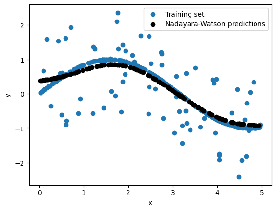
plt.scatter(X_train,y_train, label='Training set')
plt.scatter(X_test, y_pred , c="black", label = 'Nadayara-Watson predictions')
plt.xlabel('x')
plt.ylabel('y')
plt.legend()