The Poisson distribution is everywhere in biology. Examples include modeling species diversification using ODEs, the expected number of substitutions in a branch of a phylogenetic tree, and ecological count data. From a stochastic process perspective, it gives rise to Renewal and Queue theory. Here, the goal is to get a foundational understanding of the Poisson regression. Unlike continuous and binary outcome regressions, Poisson regression is usually not well covered in standard machine learning courses.
Poisson basics
The Poisson process is a discrete state and continuous time stochastic process, and its probability distribution can be seen as a special case of the Bernoulli process with a large number of trials. Assume for a period of time $t$ we have $n$ trials. Under the Poisson, the expected number of successes is $\lambda t$, over $n$ trials, the probability of success is $p = \lambda t/n$. Taking the limit of the Bernoulli probability, we have:
\[\begin{align} \lim_{n\to \infty} P(n,p) & = \lim_{n\to \infty} \binom{n}{k} p^k(1 - p)^{n-k}\\ & = \lim_{n\to \infty} \binom{n}{k} \left(\frac{\lambda t}{n}\right)^k\left(1 - \frac{\lambda t}{n}\right)^{n-k}\\ & = \lim_{n\to \infty} \frac{n \cdots (n-k) \cdots 1}{(n-k)! k!} \frac{(\lambda t)^k}{n^k} \left(1 - \frac{\lambda t}{n}\right)^{n-k}\\ & = \lim_{n\to \infty} \frac{n \cdots (n-k+1)}{n^k} \frac{(\lambda t)^k}{k!} \left(1 - \frac{\lambda t}{n}\right)^{n-k}\\ & = \lim_{n\to \infty} \frac{n}{n} \cdots \frac{n-k+1}{n} \frac{(\lambda t)^k}{k!} \left( e^{-\frac{\lambda t}{n}}\right)^{n-k} \end{align}\]Applying the limit at every term we have:
\[\begin{align} P\left(\text{Poi}(\lambda t) = k\right) := \lim_{n\to \infty} P(n,p) = \frac{(\lambda t)^k}{k!} e^{-\lambda t} \end{align}\]Considering the above, for a small interval of time $\delta$, we can approximate the probability of one event occurring in that interval as follows:
\[\begin{align} P\left(\text{Poi}(\lambda \delta) = 1\right) & = \lambda \delta \, e^{-\lambda \delta} \\ & = \lambda \delta \left( 1 - \lambda \delta + \frac{(\lambda \delta)^2}{2!} + \cdots \right) \\ & = \lambda \delta \left( 1 - \lambda \delta + o(\delta^2) \right)\\ & = \lambda \delta + o(\delta^2) \end{align}\]The fact that the probability of a given event is a small interval times the rate has found many applications in diversification modelling. Likewise, the probability of no event is:
\[\begin{align} P\left(\text{Poi}(\lambda \delta) = 0\right) & = e^{-\lambda \delta} \\ & = 1 - \lambda \delta + o(\delta^2) \end{align}\]We can also show that the probability of more than one event is negligible at this small interval:
\[\begin{align} P\left(\text{Poi}(\lambda \delta) \geq 2 \right) & = 1 - P\left(\text{Poi}(\lambda \delta) \lt 2 \right)\\ & = 1 - \left\{ P\left(\text{Poi}(\lambda \delta) = 0 \right) + P\left(\text{Poi}(\lambda \delta) = 1 \right) \right\}\\ & = 1 - \left\{ 1 - \lambda \delta + o(\delta^2) + \lambda \delta + o(\delta^2) \right\}\\ & = o(\delta^2) \end{align}\]Poisson regression framework
Let $y_i \in \mathbb{N}_0$ be a Poisson distributed random variable, that is $y_i \sim \text{Poi}(\mu_i)$, such that its probability function is given by:
\[P\left(\text{Poi}(\mu_i) = y_i\right) = \frac{(\mu_i)^{y_i} e^{-\mu_i}}{y_i!} \propto (\mu_i)^{y_i} e^{-\mu_i}\]Let $\beta \in \mathbb{R}^p$ be a column vector with a uniform distribution (i.e., flat prior) such that the Maximum A Posteriori (MAP) is equivalent to the Maximum Likelihood Estimator (MLE):
\[\begin{align} \max P\left(\beta \mid \mathbf{y}\right) & \propto \max P\left(\mathbf{y} \mid\beta \right) P\left(\beta \right)\\ & \propto \max P\left(\mathbf{y} \mid\beta \right) \\ & = \max P\left(\{\text{Poi}(\mu_i) = y_i\}_{i = 1}^{n} \mid \beta\right) \end{align}\]Non-flat priors on $\beta$ (e.g., Gaussian distributed) generally provide a regularization effect into the regression. Assuming all observations are indepedent and identical distributed (i.i.d.), we define the following objective function:
\[\begin{align} \max P\left(\{\text{Poi}(\mu_i) = y_i\}_{i = 1}^{n} \mid \beta\right) & = \max \prod_{i}^n P\left(\text{Poi}(\mu_i) = y_i \mid \beta \right) \\ & \propto \max \prod_{i}^n (\mu_i)^{y_i} e^{-\mu_i}\\ \implies \max \log P\left(\beta \mid \mathbf{y}\right) & \propto \sum_{i=1}^n y_i \log \mu_i - \mu_i \end{align}\]Since $\mu_i$ range belong to the non-negative reals, we need a link function that effectivelly maps the $\mu_i$ to all the reals such that it can be modeled by the linear function $\mathbf{x}_i^{\top}\beta$. For a Poisson distributed random variables the link function is:
\[\log (\mu_i) = \mathbf{x}_i^{\top}\beta \Longleftrightarrow \mu_i = e^{\mathbf{x}_i^{\top}\beta}\]Let our objective function be called $\mathcal{L}$:
\[\begin{align} \mathcal{L}_1 & = \sum_{i=1}^n y_i \mathbf{x}_i^{\top}\beta - e^{\mathbf{x}_i^{\top}\beta} \end{align}\]Obtaining the derivative of $\mathcal{L}_1$ with respect to $\beta$ we have:
\[\begin{align} \frac{\partial \mathcal{L}_1 }{\partial \beta} & = \sum_{i=1}^n y_i \mathbf{x}_i - \mathbf{x}_ie^{\mathbf{x}_i^{\top}\beta}\\ & = \sum_{i=1}^n \mathbf{x}_i \left( y_i - e^{\mathbf{x}_i^{\top}\beta} \right)\\ & = \begin{bmatrix} | & & |\\ \mathbf{x}_1 & \dots & \mathbf{x}_n\\ | & & | \end{bmatrix} \begin{bmatrix} y_1 - e^{\mathbf{x}_1^{\top}\beta}\\ \vdots\\ y_n - e^{\mathbf{x}_n^{\top}\beta}\\ \end{bmatrix}\\ & = \mathbf{X}^{\top}(\mathbf{y} - \boldsymbol{\mu}) \end{align}\]Now, recall that the Poisson process expectation is a function of the rate and time: $\mu_i = \lambda_i t_i$, where $\lambda_i$ is the rate of the process. It turns out that we can also model this rate using the regression framework, which gives us the following equivalence:
\[\log\left( \lambda_i \right) = \log\left( \frac{\mu_i}{t_i} \right) = \mathbf{x}_i^{\top}\beta \Longleftrightarrow \mu_i = t_i e^{\mathbf{x}_i^{\top}\beta}\]Here $e^{\mathbf{x}_i^{\top}\beta}$ implicitly models the rate $\lambda_i$. The new objective function would be:
\[\begin{align} \mathcal{L}_2 & = \sum_{i=1}^n y_i \log \left( t_i e^{\mathbf{x}_i^{\top}\beta} \right) - t_i e^{\mathbf{x}_i^{\top}\beta}\\ & = \sum_{i=1}^n y_i \left( \log t_i + \mathbf{x}_i^{\top}\beta \right) - t_i e^{\mathbf{x}_i^{\top}\beta}\\ \end{align}\]Obtaining the derivative of $\mathcal{L}_2$ with respect to $\beta$:
\[\begin{align} \frac{\partial \mathcal{L}_2 }{\partial \beta} & = \sum_{i=1}^n y_i \mathbf{x}_i - t_i \mathbf{x}_ie^{\mathbf{x}_i^{\top}\beta}\\ & = \sum_{i=1}^n \mathbf{x}_i \left( y_i - t_ie^{\mathbf{x}_i^{\top}\beta} \right)\\ & = \begin{bmatrix} | & & |\\ \mathbf{x}_1 & \dots & \mathbf{x}_n\\ | & & | \end{bmatrix} \begin{bmatrix} y_1 - t_1 e^{\mathbf{x}_1^{\top}\beta}\\ \vdots\\ y_n - t_n e^{\mathbf{x}_n^{\top}\beta}\\ \end{bmatrix}\\ & = \mathbf{X}^{\top}(\mathbf{y} - \boldsymbol{\mu}) \end{align}\]We can take the second derivative of $\mathcal{L}$ with respect to $\beta^{\top}$ to obtain the Hessian matrix and then apply the Newton-Raphson algorithm to find the optimal value of $\beta$.
Let’s take the second derivate from $\mathcal{L}_1$ to get the Hessian matrix as follows:
\[\begin{align*} \frac{\partial^2 \mathcal{L}_1}{ \partial \beta \partial \beta^{\top}} & = \frac{\partial}{\partial \beta^{\top}} \left( \sum_{i = 1}^n y_i\mathbf{x}_i - \mathbf{x}_i e^{\mathbf{x}_i^{\top}\beta} \right)\\ & = -\sum_{i = 1}^n \mathbf{x}_i \left( \frac{\partial}{\partial \beta^{\top}} e^{\mathbf{x}_i^{\top}\beta} \right) \end{align*}\]For the derivative in the $i$ term of the above summation we have:
\[\begin{align*} \frac{\partial}{\partial \beta^{\top}} e^{\mathbf{x}_i^{\top}\beta} & = \begin{bmatrix} \frac{\partial}{\partial \beta_1} e^{\mathbf{x}_i^{\top}\beta} & \cdots & \frac{\partial}{\partial \beta_p} e^{\mathbf{x}_i^{\top}\beta} \end{bmatrix}\\ & = \begin{bmatrix} x_{i,1} e^{\mathbf{x}_i^{\top}\beta} & \cdots & x_{i,p} e^{\mathbf{x}_i^{\top}\beta} \end{bmatrix}\\ & = e^{\mathbf{x}_i^{\top}\beta} \, \mathbf{x}_i^{\top} \end{align*}\]It follows that the second derivative of $\mathcal{L}_1$ is:
\[\begin{align*} \frac{\partial^2 \mathcal{L}_1}{ \partial \beta \partial \beta^{\top}} & = -\sum_{i = 1}^n \mathbf{x}_i \, e^{\mathbf{x}_i^{\top}\beta} \, \mathbf{x}_i^{\top}\\ & = -\begin{bmatrix} | & & |\\ \mathbf{x}_1 & \dots & \mathbf{x}_n\\ | & & | \end{bmatrix} \begin{bmatrix} e^{\mathbf{x}_1^{\top}\beta}\mathbf{x}_1^{\top} \\ \vdots \\ e^{\mathbf{x}_n^{\top}\beta}\mathbf{x}_n^{\top} \\ \end{bmatrix}\\ & = - \mathbf{X}^{\top} \begin{bmatrix} e^{\mathbf{x}_1^{\top}\beta} & \cdots & 0\\ \vdots & \ddots & \vdots\\ 0 & \cdots & e^{\mathbf{x}_n^{\top}\beta} \end{bmatrix} \mathbf{X}\\ & = - \mathbf{X}^{\top} \mathbf{A} \, \mathbf{X}\\ \end{align*}\]Where $\mathbf{A} \in \mathbb{R}^{n \times n}$ is a diagonal matrix with elements containing the variance of the estimator, which happens to be also the mean in the Poisson distribution.
The Newton-Raphson algorithm to find the optimal value of $\beta$ is as follows:
- Initialize $\beta$
- Repeat until convergence:
Code implementation
Data simulation:
import numpy as np
np.random.seed(12038)

n = 400
X = np.ones((n, 2))
X[:, 1] = np.random.normal(size=n)
beta = np.random.normal(size=2)
mu = np.exp(X @ beta)
y = np.random.poisson(mu)

test_idx = np.random.choice(range(n), size = int(n*0.5), replace=False)
train_idx = list( set(range(n)) - set(test_idx) )

X_train, X_test = X[train_idx,:], X[test_idx,:]
y_train, y_test = y[train_idx]  , y[test_idx]
Poisson regression using Newton-Raphson:
def poisson_reg(X, y, max_iter=100):
    _,p = X.shape
    b = np.zeros(p)
    f_old = X @ b
    for _ in range(max_iter):
        mu = np.exp(f_old)
        # Gradient and Hessian
        G = X.T @ ( y - mu )
        H = - X.T @ ( mu[:, None] * X )
        # Newton-Raphson update
        b -= np.linalg.solve(H, G)
        # Check convergence
        f_new = X @ b
        f_max = np.max(np.abs(f_new))
        f_diff = np.max(np.abs(f_new - f_old))
        if f_diff/f_max < 1e-6:
            break
        f_old = f_new

    return b
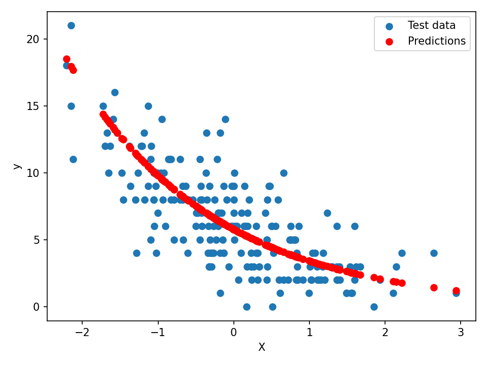
Make predictions and visualize results:
beta_hat = poisson_reg(X_train, y_train)
y_pred = np.exp(X_test @ beta_hat)

import matplotlib.pyplot as plt
plt.scatter(X_test[:, 1], y_test, label='Test Data')
plt.scatter(X_test[:, 1], y_pred, color='red', label='Predictions')
plt.xlabel('X')
plt.ylabel('y')
plt.legend()
plt.tight_layout()
References
- Lefebvre, M. (2007). Applied stochastic processes. New York, NY: Springer New York.
- Bertsekas, D., & Tsitsiklis, J. N. (2008). Introduction to probability (Vol. 1). Athena Scientific.