The likelihood of a tree

Consider the following tree:

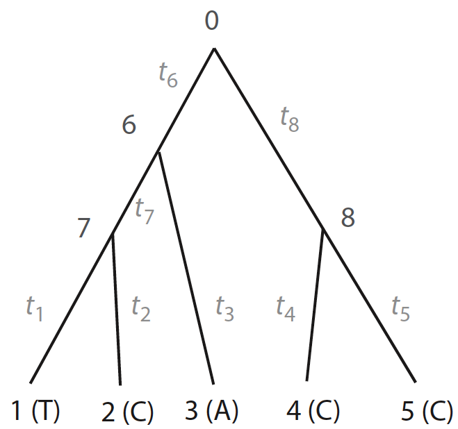
Figure 1. Tree from Yang 2014, pp. 103

Nodes from 1 to 5 can depict nucleotides of each species on a given alignment, whose states are known (\(T, C, A ,C, C\)), and nodes 0, 6, 7, and 8 depict internal nodes, whose ancetral states are unknown (\(x_{0}, x_{6}, x_{7}, x_{8}\)). Assuming that evolution is independent in both sites and lineages, the likelihood of the whole tree is given by the product between likelihood of the site \(\textbf{x}_{i}\) (i.e., node state at the root) given model parameters \(\theta\) (e.g., branch lengths, transition/transversion rate ratios):

Where \(f(x)\) is a function that calculates the likelihood node states. If we apply logarithms to both sides of the above equation we have:

Then, we just need to define \(f(x)\) and sum all terms of the right side of above equations to get the overall log-likelihood of the tree.

The pruning algorithm

The function \(f(x)\) can be defined as the sum over all possible combinations of nucleotide change probability from tips to \(x_{0}\):

Where \(\pi_{x_{0}}\) is the stationary probability (e.g., 0.25 for the K80 model), \(P_{i,j}(t)\) is the probability of base change \(i \rightarrow j\) (or \(i \leftarrow j\) due to reversebility of most DNA evolution models) along the branch length \(t\), obtained from the \(Q\) matrix (see below). While the above equation is enough to start estimating site likelihoods, the equation is not computationally efficient. For example, let expand the summation of all states in \(x_{8}\) (i.e., \(A, G, C, T\)):

We should have 8 multiplications (i.e., number of nodes - 1) for each base (i.e., 4) and 3 additions (i.e., number of bases - 1). If we denote \(s\) the number of species and \(b\) the number of bases, then the number of operations after completely expading above equation is \((2sb - b - 1)b^{s - 2}\). For our tree the number of operations then would be \((2(5)(4) - 4 - 1)4^{5 - 2} = 2240\) per site; for s = 20 it is 10,651,518,894,080

The number of operations is huge due to the number of repeated calculations. However, these repeated calculations can be avoided by factorizing the summation:

Above factorization is analogous to the factorization of \(x^2 + x\) into \(x(x + 1)\). It might not be apparent at the first sight, but above summation follows the (recursive) shape of the tree. This is the Felsenstein prunning algorithm, which is essentially a recursive algorithm.

Transition probability matrix

The probability of a base change takes the form of a Markov matrix (i.e., all elements $\geq 0$, all columns add to 1):

And a property of the Markov process is \(\mathbf{P}(t_{1} + t_{2}) = \mathbf{P}(t_{1})\mathbf{P}(t_{2}) = \mathbf{P}(t_{2})\mathbf{P}(t_{1})\) (Chapman-Kolgomorov equation). If we substract \(\mathbf{P}(t_{1})\) at both sides we have:

Notice that the identity matrix \(\textbf{I}\) is equivalent to \(\mathbf{P}(0)\) as it is a diagonal of ones, thus no base change. Then, substituting \(\mathbf{P}(0)\) into above equation and applying limits with respect of \(t_{2}\):

Letting \(t_2\) be \(\Delta t\), and putting a more straightforward format at the right hand side of above equation:

The rate of change of the probability matrix at \(t = 0\), \(\mathbf{P}^{\prime}(0)\), is also know as the \(\textbf{Q}\) matrix or instantaneous rate of change. We end up having the general form for matrix differentiation:

Approximated solution

The general solution of a matrix differentiation for any \(t\) is (see Box 1 for more details):

Then, we can approximate \(\mathbf{P}(t)\) with the following expansion of the exponential of a matrix:

Observations: i) \(\mathbf{P}(t)\) is in function of time and the initial value \(\textbf{Q}\), ii) \(\textbf{Q}\) contains information of the evolutionary model, iii) while above summation converges into a specific matrix in function of the number of terms considered, spectral decomposition could also be used when the matrix $\mathbf{Q}$ is positive semidefinite, a property seen in time-reversible Markov processes:

where $\mathbf{U}$ and $\mathbf{\Lambda}$ are the matrices of eigenvectors and eigenvalues, respectively. For instance, in models such as GTR, where $\mathbf{Q}$ is not necessarily symmetric, spectral decomposition remains applicable because $\mathbf{Q}$ can be expressed as the product of two symmetric matrices (Felsenstein 2004, pp. 206; Zhang 2014, pp. 67). For non-time-reversible Markov processes, an algorithm called scaling and squaring, which is based on the first two terms of the expansion of \(e^{ \textbf{Q}t }\), is preferred (Zhang 2014, pp. 66).

Exact solution

There are some cases where exact solution can be obtained without the need of numerical optimization over the Q matrix. This is the case of Jukes-Cantor (JC) and Kimura-2-parameters (K2P) models. Here is the solution for the K2P model:

Where transition/transversion ratio is given by \(k = \alpha/\beta\) and the coefficient \(d = (\alpha + 2\beta)t\) is a used as a proxy of time/distance between two bases. To obtain the full solution for the K2P model, the so-called ‘integrating factors’ trick should be used in the middle of the derivations.

Python implementation

Under the K2P model with \(k = 2\), if we let a branch length be \(0.2\), then the probability transition matrix can be represented as:

For this Python implementation, we assume that all leaf branches are \(0.2\), internal branches are \(0.1\), and \(k = 2\) is fixed.

Let’s focus on node \(7\) of Fig. 1. The probabilities for each base at node \(7\), derived from tip \(1\) (T) and tip \(2\) (C), are as follows:

This can also be rewritten in terms of probability vectors:

where \(\odot\) represents element-wise multiplication. Notice that \(\mathbf{L}_{x}\) and \(\mathbf{L}_{y}\) can, in turn, be rewritten as:

Here, \(\mathbf{L}_{1}\) and \(\mathbf{L}_{2}\) represent the one-hot encoding row vectors for T at node \(1\) and C at node \(2\), respectively. Then, \(\mathbf{L}_{7}\) at parent node \(7\) can be expressed in terms of the children’s probability vectors and the transition matrix \(\mathbf{P}\):

Generally, for a parent node \(k\) and child nodes \(i\) and \(j\), with branch lengths \(t_i\) and \(t_j\), respectively, we have the following recursive relation:

From there, it follows the Felsenstein pruning algorithm. As mentioned above, we are fixing the branch lengths and the substitution parameter. Determining the branch lengths and substitution parameters given a tree toplogy requires further derivations (e.g., second-order optimization of the likelihood function), which are not straightforward from the above derivations. This will be the focus of another blog post. For now, by fixing all these parameters, here is a possible implementation of the tree’s likelihood.

Kimura’s two-parameters

import math
import numpy as np

Kimura’s two-parameters equation for comparing two bases (\(i, j\)):

def k2p(i, j, d, k):
    _lib = {
        'A': 'G', 'G': 'A',
        'T': 'C', 'C': 'T'
        }
    first_t =lambda d,k:math.exp(-4*( d/(k+2) ))
    second_t=lambda d,k:2*math.exp(-2*( d*(k+1)/(k+2) ))
    
    if i == j:
        # equal base
        return 0.25*(1 + first_t(d,k) + second_t(d,k))
    else:
        if _lib[i] == j:
            # transition
            return 0.25*(1 + first_t(d,k) - second_t(d,k))
        else:
            # transversion
            return 0.25*(1 - first_t(d,k))

P matrix implementation:

def P_mat(d,k):
    """
    P matrix
    """
    bases = ['T', 'C', 'A', 'G']
    return np.array([
                [k2p(bases[0], i, d, k) for i in bases],
                [k2p(bases[1], i, d, k) for i in bases],
                [k2p(bases[2], i, d, k) for i in bases],
                [k2p(bases[3], i, d, k) for i in bases]
            ])

Here is a possible tree representation in Fig. 1:

tree = {   
  0: {'L': None, 'daughters': [6, 8], 'parent': None, 'blen': 0.0},
  1: {'L': [1, 0, 0, 0], 'daughters': [], 'parent': 7, 'blen': 0.2},
  2: {'L': [0, 1, 0, 0], 'daughters': [], 'parent': 7, 'blen': 0.2},
  3: {'L': [0, 0, 1, 0], 'daughters': [], 'parent': 6, 'blen': 0.2},
  4: {'L': [0, 1, 0, 0], 'daughters': [], 'parent': 8, 'blen': 0.2},
  5: {'L': [0, 1, 0, 0], 'daughters': [], 'parent': 8, 'blen': 0.2},
  6: {'L': None, 'daughters': [3, 7], 'parent': 0, 'blen': 0.1},
  7: {'L': None, 'daughters': [1, 2], 'parent': 6, 'blen': 0.1},
  8: {'L': None, 'daughters': [4, 5], 'parent': 0, 'blen': 0.1}, 
}

Recursive function

Via a Depth-First Search style

def dfs(n):
    print(n)
    daughters = tree[n]['daughters']
    if daughters:
        left, right = daughters
        dfs(left)
        dfs(right)
        # calculate children's likelihoods
        t_l = tree[left]['blen']
        t_r = tree[right]['blen']
        Lx = tree[left]['L'] @ P_mat(t_l, 2)
        Ly = tree[right]['L'] @ P_mat(t_r, 2)
        # calculate ancestor's likelihoods
        tree[n]['L'] = Lx * Ly

Let’s run this function from the node 0

dfs(0)
0
6
3
7
1
2
8
4
5

Now, if we see our tree after the recursive calls:

print(tree)

{0: {'L': array([1.12371115e-04, 1.83822624e-03, 7.51370241e-05, 1.36379296e-05]),
  'daughters': [6, 8],
  'parent': None,
  'blen': 0.0},
 1: {'L': [1, 0, 0, 0], 'daughters': [], 'parent': 7, 'blen': 0.2},
 2: {'L': [0, 1, 0, 0], 'daughters': [], 'parent': 7, 'blen': 0.2},
 3: {'L': [0, 0, 1, 0], 'daughters': [], 'parent': 6, 'blen': 0.2},
 4: {'L': [0, 1, 0, 0], 'daughters': [], 'parent': 8, 'blen': 0.2},
 5: {'L': [0, 1, 0, 0], 'daughters': [], 'parent': 8, 'blen': 0.2},
 6: {'L': array([0.00300556, 0.00300556, 0.00434364, 0.00044365]),
  'daughters': [3, 7],
  'parent': 0,
  'blen': 0.1},
 7: {'L': array([0.06953344, 0.06953344, 0.00205366, 0.00205366]),
  'daughters': [1, 2],
  'parent': 6,
  'blen': 0.1},
 8: {'L': array([0.00710204, 0.68077648, 0.00205366, 0.00205366]),
  'daughters': [4, 5],
  'parent': 0,
  'blen': 0.1}}

Finally, the likelihood of a particular tree is given by the probability vector for the root (i.e., tree[0]['L'] above), multiplied by the equilibrium distribution $\pi$, which is 1/4 in both the K2P and JC models:

This can be simply implemented in code as:

sum(0.25 * tree[0]['L'])
# Likelihood: 0.0005098430765880512

References

1. Yang, Z. (2014). Molecular evolution: a statistical approach. Oxford University Press.
2. Felenstein, J. (2004). Inferring phylogenies. Sunderland, MA: Sinauer associates.
3. Pupko, T., & Mayrose, I. (2020). A gentle introduction to probabilistic evolutionary models.